Conway’s Game Of Life : A Cellular Automaton

New day!! new things to learn. In this article I will be explaining all the theories that you will need to understand Conway’s Game Of Life and finally some of my own implementation-al twists more on that later. To understand Conway’s theory there are many things that you need to put your nose upfront.

Evolution Process In Conway’s Game Of Life

To start with an interesting note , Conway’s Game Of Life is a zero-player game. Yes, you are reading it right. You will have no interaction with this game. But the fun part it you get to witness the evolution process , again more on that later.

Game of life is also refereed as a cellular automaton. What is cellular automaton ? Consider it as a regular grid of cells where every cell are in one of a finite number of states. Consider (for now) this state as dead or alive, on or off , or any other Boolean logic that you can think of.

Diving deeper the current state of each cell is determined according to the state of the cells surrounding it . These set of cells are known as its neighborhood. So every cells are at a particular state initially (time t=0) and for every iteration or for every movement forward in time , new generation of cells are generated with respect to the cells in previous state (time t = t — 1). You might have a question on how do we update the cell states. Typically there are rules for updating the state of cells which applies to all cells in the grid. There are lots of other information’s about cellular automation found here in Wikipedia

Rules

The universe (environment) of the game is infinite with two dimensional orthogonal (linear) grid of square cells. These cells have a particular state at particular point of time. Every cells probability to live in next generation (another point of time (t) )depends on the present state of cells surrounding it. The decision that the cell will live or die are taken using following references:

1. Any live cell with fewer than two live neighbors dies, as if by under-population.
2. Any live cell with two or three live neighbors live on to the next generation.
3. Any live cell with more than three live neighbors dies, as if by overpopulation.
4. Any dead cell with exactly three live neighbors becomes a live cell, as if by reproduction.

Not only in this game the above mentioned rules can be seen in real life too. No-wonder it’s called Game Of Life (duhhhh)

Background

Before Conway’s Game Of Life earned its popularity, computer generated fractals were popular back then. Unlike fractal arts being a way to use wasted CPU cycles , Game of life had more philosophical impact. In the late 40’s John von Neumaan was searching an insight on use of electromagnetic components floating randomly in liquid or gas which back then was an impossible idea due to lack of superior technologies. Many researches went side by side but a gentleman namely “John Conway” initiated his own research with a variety of two dimensional cellular automaton rules which we now call “Conway’s Game Of Life”. This research by Conway was so effective that it had satisfied von Neumaan’s two general requirements.

The idea put forward by Conway were:

1. There should be no explosive growth
2. There should exist small initial patterns with chaotic, unpredictable outcomes.
3. The rules should be as simple as possible .

Since the publication of Conway’s research “Game Of Life” . It has attracted a lot of attention as it makes us able to witness, how patterns evolve.

All About Patterns

Till now different types of patterns have been discovered and are classified according to their behavior. The main motivation of researching these patterns is to determine what is the time taken by the pattern to stabilize itself. Some patterns do stabilize and some don’t or takes like gazillion CPU cycles. Most commonly found patterns are still life’s , oscillators and spaceship. To know more about Conway’s Game Of Life visit Stanford.

To visualize these different patterns there is an open source program called Golly. I don’t know much about it’s availability on other OSes but on a Debian based distribution all you need to do is

sudo apt install golly -y

To find what suits your OS visit sourceforge to download Golly from their official site.

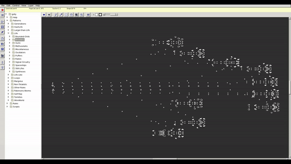
Breeding Patterns In Golly

Coding

Finally! The fun part. There are plethora of implementation for Conway’s Game Of Life. To make it more interesting I will be adding evolution that starts from an image(huh?!!). In more simple form I will take an image and process that image to generate initial state and evolve from that state and see what we end up with.

As usual the source code to my version of implementation can be found on my GitHub repository Game-Of-Life

Lets Get Started!! So the libraries you will require down the line are:

1. of-course python installed (I used python 3.9)
2. Numpy
3. Cv2
4. Matplotlib

I have divided coding part according to two different problem statement:

1. Read an image
2. Apply Games of life on the pattern from image

Image Processing

So for tackling the first problem statement, I initiated by importing following libraries

import numpy as np
import os
import cv2

After that I created a class namely RGBto2D

class RGBto2D:
    def __init__(self, name, save=False):
        self.path = os.getcwd() + '/images/' + name
        self.gray = None
        self.bw = None
        self.save = save

Here __init__() (constructor) takes two different parameters i.e name of the image file and save as to save the scaled image locally.

def to_array(self):
    image = cv2.imread(self.path, cv2.IMREAD_GRAYSCALE)
    image = cv2.resize(image, dsize=(500, 500))
    self.gray = np.array(image)

In this to_array() method we read an image using CV2 library and transform that image into gray scale so that extra overhead are eliminated. It would take light years(xd) if we did it on RGB image. After we convert that image into Gray Scale we resize them to 500 * 500 array(Which I regret already because it takes a lot of computation. My poor CPU!! lol nahh piece of pie for my 5900x *flexing). After that we simply add the newly resized array to self.gray

def to_bw(self):
    bw = np.array(self.gray).copy()
    bw[bw < 128] = 0
    bw[bw >= 128] = 1
    self.bw = bw

As I have mentioned earlier in the theoretical(boring) part that we need each cell to be either alive or dead . So here 0 applies to cell being in a dead state and 1 for being alive. Since we have converted our image into gray scale , each pixel takes in a value ranging from 0 to 255. For our “Game Of Life” theory to work we need only two logic’s. Hence the value that are less than 128 are overwritten by zeros and greater or equal by ones.

Before And After Scaling The Image

Note: The image with 0 ,1 cant be shown because the color difference between 0–1 is very hard to differentiate with our naked eyes(meaning: makes you color blind temporarily lol).

def get_bw(self):
    self.to_array()
    self.to_bw()
    if self.save:
        bw = np.array(self.gray).copy()
        bw[bw < 128] = 0
        bw[bw >= 128] = 255
        cv2.imwrite(os.getcwd() + '/images/' + 'new.png.webp', bw)
    return self.bw

get_bw() is a normal function which starts the pipeline for generating a black and white image. So first it calls to_array() function which reads and resizes the image and then calls to_bw() function which converts the pixels to fit our logic. And if save was passed as true it copies the value from self.gray and saves it locally.

Game Of Life

Now the main logic starts for “Game Of Life”

Firstly we create a class namely GameOfLife

class GameOfLife:
    def __init__(self, dpi=10, size=50, save=False, image=None):
        self.dpi = dpi
        self.grid = None
        self.fig = None
        self.ax = None
        self.im = None
        self.ON = 1
        self.OFF = 0
        self.fig_size = None
        self.size = size
        self.save = save
        self.image = image

While creating an object of this(GameOfLife) class it takes few parameters,

dpi: to define the size of each square or cells

size: this program works even if we don’t pass an image in other word it works as regular Game Of Life program if image is not present. So size being number of rows and columns.

save: a boolean variable that enables program to know if the output is to be saved locally

image: as its name suggest ,name of the image to be processed

Other variables will be tackled further down in the code

def create_grid(self):
    if self.image is not None:
        img = RGBto2D(self.image, save=True).get_bw()
        self.size = img.shape[0]
        self.grid = img
    else:
        self.grid = np.zeros((self.size, self.size))

create_grid()’s main job is to initialize the grid where each cell reside. In other words create a array with N * N size where N * N being the number of total cells required.

Here, If the image name is passed it initialize the grid according to the returned shape of the image array (i.e 500 * 500) and sets the grid as an array of Black and White image. If not then it initializes the grid as array of zeros which we will randomize later. So, if image is present there is no randomization.

def randomize(self):
    random = np.random.random((2, 2))
    self.grid[0:2, 0:2] = (random > 0.75)

To generate random pattern, here we generate an array with size 2*2 with random values and we replace the randomly generated array inside the grid.

( the size can be any it is not mandatory to be 2 2*)

def set_fig(self):
    self.fig, self.ax = plt.subplots()
    self.im = self.ax.imshow(self.grid, interpolation='nearest')

Since I will not be teaching how to use Matplotlib take this function as a mechanism to prepare a canvas (Picasso Mode ON!! ).

def count_neighbors(self, x, y):
    count = 0
    for i in range(-1, 2, 1):
        for j in range(-1, 2, 1):
            if (i != 0) or (j != 0):
                row = (x + i) % self.size
                col = (y + i) % self.size
                count += self.grid[row, col]
    return count

“Game of life” completely works on the mechanism of a particular cells neighbor being dead or alive. We do no different in this count_neighbors() method. Here we take a cell namely x,y and iterate over its preceding and exceeding cells or neighbors. Initially the neighbor count is 0 as we haven’t visited any other cells.

You might ask why are we iterating through -1 to 1 only. It’s that the logic!! neighbor of a cell is either behind , forward , top or bottom of it. So, a cell has eight neighbors.

Again, You might think if in that case why do we iterate nine(9) time . Look carefully! If both i and j are 0 it is skipped because a cell’s current state has no significance on it’s upcoming state. Since, our array is initialized as 0 or 1 we simply add the value inside it’s neighboring cells. So, total neighbor count is the sum of total neighboring cells alive.

(x + i) % self.size

The above mentioned logic((x + i) % self.size) helps us to overcome edge cases. The cells on topmost , bottom-most, rightmost and leftmost has less neighbors in comparison to other cells.

For Example :

If we are trying to find the neighbors of rightmost cells then their exceeding cells are out of reach because array does not reference (N + 1) cells where N being size of an array. So, to prevent array index out of bound from happening we implement the above mention logic. Consider last row as 49 so (49 + 1) = 50 which is its exceeding neighbor. Since array starts indexing first cell from 0 there is no such index as 50 . So now we do 50 % size (i.e 50) which gives 0. Magic! Problem solved.

def animate(self, frame):
    print(frame)
    new_grid = self.grid.copy()
    for row in range(self.size):
        for col in range(self.size):
            neigh = self.count_neighbors(row, col)

            if self.grid[row, col] == self.ON:
                if (neigh < 2) or (neigh > 3):
                    new_grid[row, col] = self.OFF
            else:
                if neigh == 3:
                    new_grid[row, col] = self.ON

    self.im.set_data(new_grid)
    self.grid = new_grid
    return self.im,

This function namely animate() is called to generate next state of cells. It is called with respect to the frames that we will initialize. So, if frame is initialized as 50 then our program will call this function 50 times . In this function, We initially copy the reference of grid(i.e present state). We then iterate over the cells to generate new states. Since, counting neighbors is tackled we here just call the respective function.

Not taking much time , What we do here is we iterate over every cell and counts its neighbor. If current cell is alive and it’s neighbor count is less than two(under population ) or greater than three (overpopulation) we set that cell as dead.

Following that if current cell is dead and its neighbor count is exactly 3 then we resurrect (fancy word meaning raise from the dead xd) that cell.

def start(self):

    self.create_grid()
    if self.image is None:
        self.randomize()
    self.set_fig()
    ani = animation.FuncAnimation(self.fig, self.animate,  
           frames=300, interval=300,save_count=10)
    if self.save:
        ani.save('demo.mp4', fps=60, extra_args=['-vcodec', 
                                                      'libx264'])

Finally, We need some function to start all these logic chronologically. start() function does no different. It firstly initializes the gird. If image is not given it randomizes the cells initialized as zeros. Then, all the mandatory function required to kick in the animation and saving the output as a video are called.

After all this effort we are blessed with a beautiful evolution video.

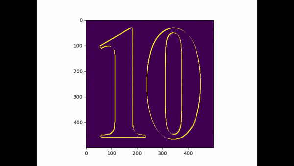
(A small tribute the G.O.A.T no 10 leo Messi)

If you are more into algorithms check my previous article on Monte Carlo Simulation and for those making their way through AI check my another article on How to Make Your Own AI Powered Game.